In this post, we demonstrate how to efficiently fine-tune a state-of-the-art protein language model (pLM) to predict protein subcellular localization using Amazon SageMaker.
Proteins are the molecular machines of the body, responsible for everything from moving your muscles to responding to infections. Despite this variety, all proteins are made of repeating chains of molecules called amino acids. The human genome encodes 20 standard amino acids, each with a slightly different chemical structure. These can be represented by letters of the alphabet, which then allows us to analyze and explore proteins as a text string. The enormous possible number of protein sequences and structures is what gives proteins their wide variety of uses.
Proteins also play a key role in drug development, as potential targets but also as therapeutics. As shown in the following table, many of the top-selling drugs in 2022 were either proteins (especially antibodies) or other molecules like mRNA translated into proteins in the body. Because of this, many life science researchers need to answer questions about proteins faster, cheaper, and more accurately.
| Name | Manufacturer | 2022 Global Sales ($ billions USD) | Indications |
| Comirnaty | Pfizer/BioNTech | $40.8 | COVID-19 |
| Spikevax | Moderna | $21.8 | COVID-19 |
| Humira | AbbVie | $21.6 | Arthritis, Crohn’s disease, and others |
| Keytruda | Merck | $21.0 | Various cancers |
Data source: Urquhart, L. Top companies and drugs by sales in 2022. Nature Reviews Drug Discovery 22, 260–260 (2023).
Because we can represent proteins as sequences of characters, we can analyze them using techniques originally developed for written language. This includes large language models (LLMs) pretrained on huge datasets, which can then be adapted for specific tasks, like text summarization or chatbots. Similarly, pLMs are pre-trained on large protein sequence databases using unlabeled, self-supervised learning. We can adapt them to predict things like the 3D structure of a protein or how it may interact with other molecules. Researchers have even used pLMs to design novel proteins from scratch. These tools don’t replace human scientific expertise, but they have the potential to speed up pre-clinical development and trial design.
One challenge with these models is their size. Both LLMs and pLMs have grown by orders of magnitude in the past few years, as illustrated in the following figure. This means that it can take a long time to train them to sufficient accuracy. It also means that you need to use hardware, especially GPUs, with large amounts of memory to store the model parameters.

Long training times, plus large instances, equals high cost, which can put this work out of reach for many researchers. For example, in 2023, a research team described training a 100 billion-parameter pLM on 768 A100 GPUs for 164 days! Fortunately, in many cases we can save time and resources by adapting an existing pLM to our specific task. This technique is called fine-tuning, and also allows us to borrow advanced tools from other types of language modeling.
Solution overview
The specific problem we address in this post is subcellular localization: Given a protein sequence, can we build a model that can predict if it lives on the outside (cell membrane) or inside of a cell? This is an important piece of information that can help us understand the function and whether it would make a good drug target.
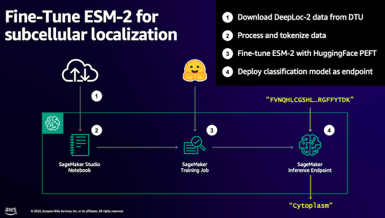
We start by downloading a public dataset using Amazon SageMaker Studio. Then we use SageMaker to fine-tune the ESM-2 protein language model using an efficient training method. Finally, we deploy the model as a real-time inference endpoint and use it to test some known proteins. The following diagram illustrates this workflow.

In the following sections, we go through the steps to prepare your training data, create a training script, and run a SageMaker training job. All of the code featured in this post is available on GitHub.
Prepare the training data
We use part of the DeepLoc-2 dataset, which contains several thousand SwissProt proteins with experimentally determined locations. We filter for high-quality sequences between 100–512 amino acids:
df = pd.read_csv(
    "https://services.healthtech.dtu.dk/services/DeepLoc-2.0/data/Swissprot_Train_Validation_dataset.csv"
).drop(["Unnamed: 0", "Partition"], axis=1)
df["Membrane"] = df["Membrane"].astype("int32")

# filter for sequences between 100 and 512 amino acides
df = df[df["Sequence"].apply(lambda x: len(x)).between(100, 512)]

# Remove unnecessary features
df = df[["Sequence", "Kingdom", "Membrane"]]
Next, we tokenize the sequences and split them into training and evaluation sets:
dataset = Dataset.from_pandas(df).train_test_split(test_size=0.2, shuffle=True)
tokenizer = AutoTokenizer.from_pretrained("facebook/esm2_t33_650M_UR50D")

def preprocess_data(examples, max_length=512):
    text = examples["Sequence"]
    encoding = tokenizer(text, truncation=True, max_length=max_length)
    encoding["labels"] = examples["Membrane"]
    return encoding

encoded_dataset = dataset.map(
    preprocess_data,
    batched=True,
    num_proc=os.cpu_count(),
    remove_columns=dataset["train"].column_names,
)

encoded_dataset.set_format("torch")
Finally, we upload the processed training and evaluation data to Amazon Simple Storage Service (Amazon S3):
train_s3_uri = S3_PATH + "/data/train"
test_s3_uri = S3_PATH + "/data/test"

encoded_dataset["train"].save_to_disk(train_s3_uri)
encoded_dataset["test"].save_to_disk(test_s3_uri)
Create a training script
SageMaker script mode allows you to run your custom training code in optimized machine learning (ML) framework containers managed by AWS. For this example, we adapt an existing script for text classification from Hugging Face. This allows us to try several methods for improving the efficiency of our training job.
Method 1: Weighted training class
Like many biological datasets, the DeepLoc data is unevenly distributed, meaning there isn’t an equal number of membrane and non-membrane proteins. We could resample our data and discard records from the majority class. However, this would reduce the total training data and potentially hurt our accuracy. Instead, we calculate the class weights during the training job and use them to adjust the loss.
In our training script, we subclass the Trainer class from transformers with a WeightedTrainer class that takes class weights into account when calculating cross-entropy loss. This helps prevent bias in our model:
class WeightedTrainer(Trainer):
    def __init__(self, class_weights, *args, **kwargs):
        self.class_weights = class_weights
        super().__init__(*args, **kwargs)

    def compute_loss(self, model, inputs, return_outputs=False):
        labels = inputs.pop("labels")
        outputs = model(**inputs)
        logits = outputs.get("logits")
        loss_fct = torch.nn.CrossEntropyLoss(
            weight=torch.tensor(self.class_weights, device=model.device)
        )
        loss = loss_fct(logits.view(-1, self.model.config.num_labels), labels.view(-1))
        return (loss, outputs) if return_outputs else loss
Method 2: Gradient accumulation
Gradient accumulation is a training technique that allows models to simulate training on larger batch sizes. Typically, the batch size (the number of samples used to calculate the gradient in one training step) is limited by the GPU memory capacity. With gradient accumulation, the model calculates gradients on smaller batches first. Then, instead of updating the model weights right away, the gradients get accumulated over multiple small batches. When the accumulated gradients equal the target larger batch size, the optimization step is performed to update the model. This lets models train with effectively bigger batches without exceeding the GPU memory limit.
However, extra computation is needed for the smaller batch forward and backward passes. Increased batch sizes via gradient accumulation can slow down training, especially if too many accumulation steps are used. The aim is to maximize GPU usage but avoid excessive slowdowns from too many extra gradient computation steps.
Method 3: Gradient checkpointing
Gradient checkpointing is a technique that reduces the memory needed during training while keeping the computational time reasonable. Large neural networks take up a lot of memory because they have to store all the intermediate values from the forward pass in order to calculate the gradients during the backward pass. This can cause memory issues. One solution is to not store these intermediate values, but then they have to be recalculated during the backward pass, which takes a lot of time.
Gradient checkpointing provides a balanced approach. It saves only some of the intermediate values, called checkpoints, and recalculates the others as needed. Therefore, it uses less memory than storing everything, but also less computation than recalculating everything. By strategically selecting which activations to checkpoint, gradient checkpointing enables large neural networks to be trained with manageable memory usage and computation time. This important technique makes it feasible to train very large models that would otherwise run into memory limitations.
In our training script, we turn on gradient activation and checkpointing by adding the necessary parameters to the TrainingArguments object:
from transformers import TrainingArguments

training_args = TrainingArguments(
	gradient_accumulation_steps=4,
	gradient_checkpointing=True
)
Method 4: Low-Rank Adaptation of LLMs
Large language models like ESM-2 can contain billions of parameters that are expensive to train and run. Researchers developed a training method called Low-Rank Adaptation (LoRA) to make fine-tuning these huge models more efficient.
The key idea behind LoRA is that when fine-tuning a model for a specific task, you don’t need to update all the original parameters. Instead, LoRA adds new smaller matrices to the model that transform the inputs and outputs. Only these smaller matrices are updated during fine-tuning, which is much faster and uses less memory. The original model parameters stay frozen.
After fine-tuning with LoRA, you can merge the small adapted matrices back into the original model. Or you can keep them separate if you want to quickly fine-tune the model for other tasks without forgetting previous ones. Overall, LoRA allows LLMs to be efficiently adapted to new tasks at a fraction of the usual cost.
In our training script, we configure LoRA using the PEFT library from Hugging Face:
from peft import get_peft_model, LoraConfig, TaskType
import torch
from transformers import EsmForSequenceClassification

model = EsmForSequenceClassification.from_pretrained(
	“facebook/esm2_t33_650M_UR50D”,
	Torch_dtype=torch.bfloat16,
	Num_labels=2,
)

peft_config = LoraConfig(
    task_type=TaskType.SEQ_CLS,
    inference_mode=False,
    bias="none",
    r=8,
    lora_alpha=16,
    lora_dropout=0.05,
    target_modules=[
        "query",
        "key",
        "value",
        "EsmSelfOutput.dense",
        "EsmIntermediate.dense",
        "EsmOutput.dense",
        "EsmContactPredictionHead.regression",
        "EsmClassificationHead.dense",
        "EsmClassificationHead.out_proj",
    ]
)

model = get_peft_model(model, peft_config)
Submit a SageMaker training job
After you have defined your training script, you can configure and submit a SageMaker training job. First, specify the hyperparameters:
hyperparameters = {
    "model_id": "facebook/esm2_t33_650M_UR50D",
    "epochs": 1,
    "per_device_train_batch_size": 8,
    "gradient_accumulation_steps": 4,
    "use_gradient_checkpointing": True,
    "lora": True,
}
Next, define what metrics to capture from the training logs:
metric_definitions = [
    {"Name": "epoch", "Regex": "'epoch': ([0-9.]*)"},
    {
        "Name": "max_gpu_mem",
        "Regex": "Max GPU memory use during training: ([0-9.e-]*) MB",
    },
    {"Name": "train_loss", "Regex": "'loss': ([0-9.e-]*)"},
    {
        "Name": "train_samples_per_second",
        "Regex": "'train_samples_per_second': ([0-9.e-]*)",
    },
    {"Name": "eval_loss", "Regex": "'eval_loss': ([0-9.e-]*)"},
    {"Name": "eval_accuracy", "Regex": "'eval_accuracy': ([0-9.e-]*)"},
]
Finally, define a Hugging Face estimator and submit it for training on an ml.g5.2xlarge instance type. This is a cost-effective instance type that is widely available in many AWS Regions:
from sagemaker.experiments.run import Run
from sagemaker.huggingface import HuggingFace
from sagemaker.inputs import TrainingInput

hf_estimator = HuggingFace(
    base_job_name="esm-2-membrane-ft",
    entry_point="lora-train.py",
    source_dir="scripts",
    instance_type="ml.g5.2xlarge",
    instance_count=1,
    transformers_version="4.28",
    pytorch_version="2.0",
    py_version="py310",
    output_path=f"{S3_PATH}/output",
    role=sagemaker_execution_role,
    hyperparameters=hyperparameters,
    metric_definitions=metric_definitions,
    checkpoint_local_path="/opt/ml/checkpoints",
    sagemaker_session=sagemaker_session,
    keep_alive_period_in_seconds=3600,
    tags=[{"Key": "project", "Value": "esm-fine-tuning"}],
)

with Run(
    experiment_name=EXPERIMENT_NAME,
    sagemaker_session=sagemaker_session,
) as run:
    hf_estimator.fit(
        {
            "train": TrainingInput(s3_data=train_s3_uri),
            "test": TrainingInput(s3_data=test_s3_uri),
        }
    )
The following table compares the different training methods we discussed and their effect on the runtime, accuracy, and GPU memory requirements of our job.
| Configuration | Billable Time (min) | Evaluation Accuracy | Max GPU Memory Usage (GB) |
| Base Model | 28 | 0.91 | 22.6 |
| Base + GA | 21 | 0.90 | 17.8 |
| Base + GC | 29 | 0.91 | 10.2 |
| Base + LoRA | 23 | 0.90 | 18.6 |
All of the methods produced models with high evaluation accuracy. Using LoRA and gradient activation decreased the runtime (and cost) by 18% and 25%, respectively. Using gradient checkpointing decreased the maximum GPU memory usage by 55%. Depending on your constraints (cost, time, hardware), one of these approaches may make more sense than another.
Each of these methods perform well by themselves, but what happens when we use them in combination? The following table summarizes the results.
| Configuration | Billable Time (min) | Evaluation Accuracy | Max GPU Memory Usage (GB) |
| All methods | 12 | 0.80 | 3.3 |
In this case, we see a 12% reduction in accuracy. However, we’ve reduced the runtime by 57% and GPU memory use by 85%! This is a massive decrease that allows us to train on a wide range of cost-effective instance types.
Clean up
If you’re following along in your own AWS account, delete the any real-time inference endpoints and data you created to avoid further charges.
predictor.delete_endpoint()

bucket = boto_session.resource("s3").Bucket(S3_BUCKET)
bucket.objects.filter(Prefix=S3_PREFIX).delete()
Conclusion
In this post, we demonstrated how to efficiently fine-tune protein language models like ESM-2 for a scientifically relevant task. For more information about using the Transformers and PEFT libraries to train pLMS, check out the posts Deep Learning With Proteins and ESMBind (ESMB): Low Rank Adaptation of ESM-2 for Protein Binding Site Prediction on the Hugging Face blog. You can also find more examples of using machine learning to predict protein properties in the Awesome Protein Analysis on AWS GitHub repository.
About the Author
 Brian Loyal is a Senior AI/ML Solutions Architect in the Global Healthcare and Life Sciences team at Amazon Web Services. He has more than 17 years’ experience in biotechnology and machine learning, and is passionate about helping customers solve genomic and proteomic challenges. In his spare time, he enjoys cooking and eating with his friends and family.


