Introduction
Recurrent Neural Networks (RNN) by design are intrinsically suited for analyzing sequences of data, such as genomes, time series, text, or even handwriting. In industry, they are found processing sequential data from stock markets or sensors, while in the digital world, they power applications like language modeling, language translation, text generation, speech recognition, video tagging, and image description generation.
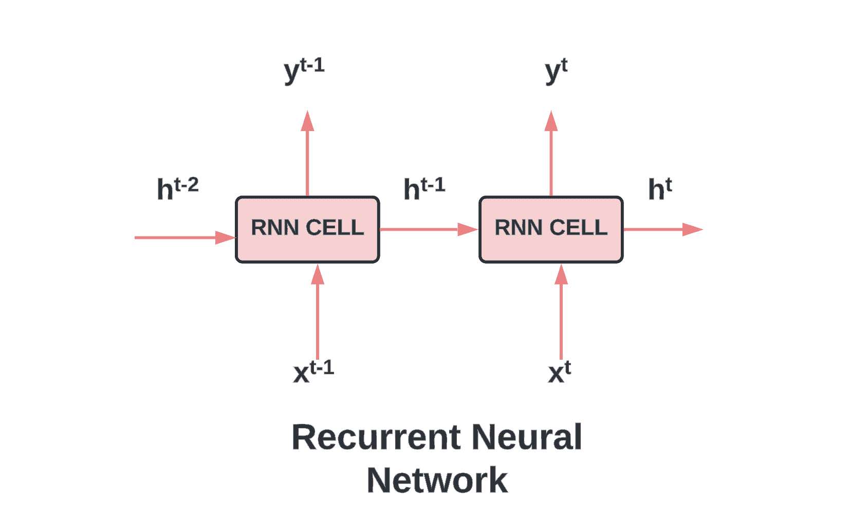
One defining feature of RNNs is their internal memory, supported by recurrent units that capture information from previous time steps, effectively incorporating past input into current and future computations. Unlike feedforward networks, recurrent networks leverage information from previous inputs, making them particularly suitable for processing sequential data.
Single input, single output, or multiple outputs, an RNN efficiently handles different configurations and the nature of the task, whether it involves forecasting the future input or classifying the input sequence.
RNN’s are known to suffer from issues like vanishing and exploding gradients when trained with long sequences. These issues are mitigated to some extent by RNN variants like Long Short-Term Memory (LSTM) and Gated Recurrent Unit (GRU) networks, which introduce gating mechanisms to better manage information flow.
What are recurrent neural networks?
Recurrent Neural Networks are a class of artificial neural networks designed to recognize patterns in sequences of data, such as text, genomes, handwriting, or the spoken word. They are called “recurrent” because they perform the same task for every element in a sequence, with the output depending on the previous computations. This is different from traditional neural networks, which process inputs independently.
Think of RNNs as a person reading a sentence. The person doesn’t start fresh with each new word – they understand the sentence’s meaning based on the context provided by the words they’ve already read. Similarly, RNNs can use their reasoning about previous events in the sequence to inform later ones. This feature makes them extraordinarily powerful for tasks involving sequential data.
The training process of RNNs employs techniques such as Backpropagation Through Time (BPTT) and Gradient Descent. The computation of error gradients and partial derivatives is fundamental to this learning process.
To illustrate this with a diagram, you would start by drawing a standard feed-forward neural network but then add arrows looping from the output of each neuron back to its input. This represents the recurrent nature of the RNN.
How recurrent neural networks learn
The learning process in an RNN involves a method known as “Backpropagation Through Time” (BPTT). In essence, BPTT works by unrolling the entire input sequence, applying standard backpropagation, and then rolling it back to its original form. The key idea behind BPTT is to treat the RNN as a deep neural network (DNN) with shared weights, as this allows the use of standard training techniques.
BPTT is a modification of the standard backpropagation algorithm used in a typical feed-forward neural network, adapted to suit the recurrent nature of RNNs. The essential idea of BPTT is to “unroll” the RNN in time, treat it as a deep neural network (DNN) with shared weights across time steps, and then apply standard backpropagation. Once the gradients are calculated, the sequence is “rolled” back up into its original recurrent form.
Consider an RNN where at each time step “t”, we have an input “x_t” and a hidden state “h_t”. The hidden state “h_t” is a function of the previous hidden state “h_{t-1}” and the current input “x_t”. This relationship can be represented with the following equation:
Here, “W” denotes the weights associated with the recurrent neurons, “U” denotes the weights for the input neurons, and “f” is an activation function like the hyperbolic tangent (tanh) or rectified linear unit (ReLU). The activation function “f” introduces non-linearity into the model, enabling the network to learn and represent complex patterns.
Now, let’s extend this formulation to the output at each time step. The output “y_t” is typically a function of the hidden state at time “t”. This can be represented as:
In this equation, “V” are the weights of the connections from the hidden layer to the output layer, and “g” is a suitable activation function for the output layer, such as softmax for a multi-class classification problem.
After defining the forward pass of the RNN, we can now proceed to understand the learning process, which involves adjusting the parameters (W, U, V) using BPTT. In the backpropagation phase, the error is propagated from the output layer back through the network to adjust the weights. This process involves computing the gradients of the loss function with respect to the parameters and then updating the parameters in the direction that minimizes the loss. The mathematical details of BPTT involve several steps of differentiation and application of the chain rule and can be quite involved.
To aid understanding, consider unrolling an RNN for an entire sequence of length T. Each time step can be thought of as a separate layer in a DNN, with the crucial difference that the weights (W, U, V) are shared across layers (i.e., time steps). This unrolled view of the RNN helps visualize the BPTT algorithm in action as it propagates errors back through the network and guides the learning of optimal weights to improve the model’s predictions over time.
The choice of activation function, such as the softmax function, and the loss function significantly influence the performance of an RNN in tasks like binary classification. Model hyperparameters such as the learning rate and the number of training epochs significantly influence the performance of the model. Batch normalization, a technique used to improve the stability and performance of neural networks, can also be applied to RNNs with considerations about batch size.
To illustrate this in a diagram, show the unrolling of the RNN for an entire sequence, where each time step is represented as a separate layer in a DNN.
Bidirectional recurrent neural networks
Bidirectional Recurrent Neural Networks (Bi-RNNs) extend the concept of traditional RNNs by introducing another layer of hidden states that processes the sequence in the reverse order. This additional layer allows the model to have access to both past (via forward states) and future data (via backward states), making them suitable for tasks where the context in both directions is needed for optimal performance.
Bi-RNNs employ two separate hidden layers. The forward layer is represented as H with a right arrow on top, and the backward layer is represented as H with a left arrow on top. The computations for these layers at time step ‘t’ are given by:
Here, W with subscript ‘x right arrow h’, W with subscript ‘right arrow hh’, W with subscript ‘x left arrow h’, and W with subscript ‘left arrow hh’ are the weight matrices, and ‘b right arrow h’ and ‘b left arrow h’ are the respective biases. The forward hidden state, represented as ‘H right arrow at time t’, and the backward hidden state, represented as ‘H left arrow at time t’, is computed with inputs ‘X at time t’ and the previous hidden states ‘H right arrow at time t-1’ and ‘H left arrow at time t+1’ respectively.
Sigma represents the activation function such as tanh or ReLU that transforms the output within a certain range. Note that in the backward layer, we use ‘H left arrow at time t+1’, meaning we are using the future state to compute the current state.
The final output ‘y at time t’ at each time step is usually computed by concatenating or adding the forward and backward hidden states, and then transforming through a dense layer:
Where W with subscript ‘right arrow hy’, W with subscript ‘left arrow hy’, and ‘b subscript y’ are the weight matrices and bias for the output layer, and the softmax function is used for normalization if the task is multi-class classification.
By incorporating future information with the backward pass, Bi-RNNs can find patterns that may be missed by regular RNNs or even LSTMs and GRUs. However, they require more computation and are not suitable for real-time predictions as they need the entire sequence beforehand to make a prediction.
RNN challenges and how to solve them
RNNs have two major issues: vanishing and exploding gradients. Both are related to the magnitudes of the gradients – quantities computed while performing backpropagation to adjust the network’s weights.
In the case of the vanishing gradients problem, the gradients can become exceedingly small. As a result, when the backpropagation algorithm adjusts the weights, the adjustments can be so minuscule that the learning becomes incredibly slow or even stops entirely.
The exploding gradients problem is the opposite. The gradients become so large that they cause drastic changes in the weights, leading the learning process to diverge and fail.
Also Read: Introduction to Radial Bias Function Networks
Long short-term memory units
To address the problem of vanishing gradients, Long Short-Term Memory units (LSTMs) were introduced. LSTMs maintain a more constant error, facilitating RNNs to learn over substantially long sequences (over 1000 time steps). They achieve this feat by storing information outside the conventional neural network flow in structures known as gated cells.
In essence, an LSTM has three of these gates, each one being a way the LSTM can choose to remember or forget certain information. They are:
- Forget Gate (F_t): Decides what information to throw away from the cell state.
- Input Gate (I_t ): Updates the cell state with new information from the current input.
- Output Gate (O_t): Decides what the next hidden state should be.
Here, σ represents the sigmoid activation function transforming the output within the range (0, 1), and W_{xo}, W_{xi}, W_{xf}, W_{ho}, W_{hi}, W_{hf} are the weight matrices and b_o, b_i, b_f are their respective biases.
In addition, LSTMs employ a candidate memory cell C~_t computed similarly to the aforementioned gates but use a tanh activation function to keep the output within the range (-1, 1):
Together these components consider old memory content C_{t-1} to control how much of the previous memory we want to retain to form the new memory content C_t. This is accomplished through element-wise multiplication, as shown:
Here, the tanh function ensures each element of H_t lies within (-1, 1).
Each of these gates involves a simple equation, similar to what we saw in the basic RNN, but combined in such a way as to enforce the LSTM’s unique capabilities.
Visualizing LSTMs can be tricky due to their complexity, but a good way to start is by drawing a box for the cell state and then separating boxes or lines for each gate, showing how they interact with the cell state.
Gated recurrent units
Gated Recurrent Units (GRUs) are a type of RNN architecture and a variation on the LSTM. GRUs combine the forget and input gates into a single “update gate.” They also merge the cell state and hidden state, and make some other changes. The result is a simpler model, although it’s not clear whether it’s categorically better or worse than the LSTM.
GRUs implement two key gates: an update gate z_t to decide how much of the previous state should be kept, and a reset gate r_t to decide how much of the previous state should be forgotten. The computations for these gates are given by:
Here, σ represents the sigmoid activation function transforming the output within the range (0, 1), and W_{xz}, W_{xr}, W_{hz}, W_{hr} are the weight matrices, and b_z, b_r are their respective biases.
In addition, GRUs employ a candidate hidden state H~_t computed similarly to the aforementioned gates but uses a tanh activation function to keep the output within the range (-1, 1):
The final hidden state H_t is a linear interpolation between the previous hidden state H_{t-1} and the candidate hidden state H~_t, with the update gate z_t deciding the ratio of mixing:
Here, the dot symbol represents element-wise multiplication.
This simpler structure is sometimes more suitable for certain tasks due to its efficiency and uses fewer computational resources. However, which type of unit is better depends heavily on the specific application, as the performances of LSTMs and GRUs are similar in many tasks.
This simpler structure is sometimes more suitable for certain tasks due to its efficiency and uses fewer computational resources. However, which type of unit is better depends heavily on the specific application, as the performances of LSTMs and GRUs are similar in many tasks.
Advantages of Recurrent Neural Network
Handling Sequential Data
RNNs’ ability to process sequential data makes them uniquely suited for time-series prediction, natural language processing, speech recognition, and more. They have what’s known as the ‘universal approximation’ property. This means they can approximate arbitrary nonlinear dynamical systems with high precision, under flexible conditions.
Flexibility
They can handle inputs and outputs of different lengths, which is particularly useful for tasks like text translation.
Shared Parameters
In RNNs, the same parameters are used for every time step of the input, which can be beneficial in terms of memory and computational efficiency.
Associative memories
One of the intriguing uses of recurrent networks is their role in building associative memories. They can construct attractors from input-output associations, which is a useful trait in many data-processing tasks. Furthermore, recurrent neural networks have found widespread use in human-robot interaction tasks, showcasing their adaptability and functionality in real-world applications.
Challenges of Recurrent Neural Network
Computational Intensity:
One limitation of RNNs is their difficulty in processing very long sequences if they’re using activation functions like tan(h) or sigmoid. These functions, although effective for normalizing input, can lead to computational difficulties for large sequences.
Difficulty with Long Sequences
Traditional RNNs struggle with longer sequences due to vanishing and exploding gradient problems.
Overfitting
Like almost all machine learning models, RNNs can suffer from overfitting, though techniques such as dropout can help with this. The nonlinear nature of unit activation output characteristics and weight adjustment strategies often makes it challenging to ascertain the network’s stability.
Applications of RNN
Despite these challenges, RNNs have been successfully applied in various unique niche:
Natural Language Processing
RNNs are commonly used in text generation, machine translation, and sentiment analysis. “Learning phrase representations using RNN encoder-decoder for statistical machine translation” by K. Cho et al. (2014). This paper proposed a novel neural network model called RNN Encoder–Decoder, which consists of two recurrent neural networks. One RNN encodes a sequence of symbols into a fixed-length vector representation, and the other decodes the representation into another sequence of symbols. This architecture was found to be effective in improving the performance of statistical machine translation systems and provided meaningful representation of linguistic phrases that preserved both the semantic and syntactic structure of the phrase
Speech Recognition
They have proven highly effective at understanding spoken language.
Time-Series Prediction: Their ability to handle sequential data makes them well-suited to financial forecasting, among other things. “Speech recognition with deep recurrent neural networks” by A. Graves (2013). This paper presented deep recurrent neural networks (RNNs) as a powerful model for sequential data like speech. The paper focused on end-to-end training where RNNs learn to map directly from acoustic to phonetic sequences, removing the need for a predefined (and error-prone) alignment to create the training targets.
Also Read: Pandas and Large DataFrames: How to Read in Chunks
Conclusion
Deep learning, of which RNN is a part, is a significant contributor to advancements in fields such as Artificial Intelligence and Reinforcement Learning. Variants of RNNs, including Long Short-Term Memory Networks (LSTMs) and Gated Recurrent Units (GRUs), enhance the model’s capacity to retain short-term memory.
Recurrent networks and feedforward networks share common components such as input and output layers, but differ in their architecture and data handling – the former processes data with sequence dependency, while the latter assumes data points are independent.
While they come with their own set of challenges, the development of gated variants like LSTMs and GRUs has largely addressed these issues. As we continue to refine these models and invent new ones, we can expect even more impressive applications of RNNs in the future.
References
Aggarwal, Charu C. Neural Networks and Deep Learning: A Textbook. Springer, 2018.
Bianchi, Filippo Maria, et al. Recurrent Neural Networks for Short-Term Load Forecasting: An Overview and Comparative Analysis. Springer, 2017.
Kostadinov, Simeon. Recurrent Neural Networks with Python Quick Start Guide: Sequential Learning and Language Modeling with TensorFlow. Packt Publishing Ltd, 2018.
Mandic, Danilo P., and Jonathon A. Chambers. Recurrent Neural Networks for Prediction: Learning Algorithms, Architectures and Stability. John Wiley & Sons, 2001.
Salem, Fathi M. Recurrent Neural Networks: From Simple to Gated Architectures. Springer Nature, 2022.


