Introduction
Keras, a popular deep-learning library, has made it simpler than ever to build and train such models. One crucial aspect of the training process is selecting the right loss function to optimize your model’s performance.
But first, let’s understand what a loss function is.
In the realm of deep learning, a loss function measures the difference between the model’s predictions and the ground truth. It is the driving force behind the training process, as it provides the gradients necessary to adjust the model’s weights through backpropagation. During each iteration, the loss is computed, and the model’s weights are updated to minimize this value. This process continues until no significant improvements in the evaluation metric are observed.
While the evaluation metric (e.g., F1 score or AUC) remains consistent throughout your machine learning project, the loss function can be fine-tuned and adapted to achieve the best performance possible. In essence, the loss function is as crucial to the success of your model as the architecture and the optimizer. Therefore, it’s important to carefully consider your options when choosing the right loss function for your problem.
A recent study explored the impacts of various loss functions on ultrasound image quality using machine learning algorithms, highlighting the importance of choosing the right loss function for specific applications (see “Impacts of Losses Functions on the Quality of the Ultrasound Image by Using Machine Learning Algorithms” in IEEE Xplore).
In this article, we’ll delve into various loss functions offered by Keras and discuss their applications, enabling you to make an informed decision when selecting the ideal loss function for your deep learning model.
Loss functions basics
In machine learning, our primary objective is to learn a function ‘f’ that maps an input space ‘Φ’ to a desired output space ‘Y’:
f : Φ → Y
To approximate this function, we use a model ‘fΘ’ parameterized by the parameters ‘Θ’. Given a set of inputs {x0, …, xN} in Φ, we train the model with corresponding target variables {y0, …, yN} in Y. In some cases, such as with autoencoders, Y is equal to Φ.
A loss function, denoted as L, quantifies the difference between the model’s predictions f(xi) and the actual target values yi by mapping them to a real number l in R. To compute the overall loss, we aggregate the loss across all data points:
L(f|{x0, …, xN}, {y0, …, yN}) = (1/N) * Σ[N, i=1] L(f(xi), yi) (1)
The optimization problem can then be expressed as:
min f L(f|{x0, …, xN}, {y0, …, yN}) (2)
In the context of our Keras loss function article, we aim to explore various loss functions that can be used to quantify the difference between predicted and actual values, ultimately helping us optimize our deep learning models.
https://chart-studio.plotly.com/~aayushmittalaayush/14/#/
Which loss functions are available in Keras?
Loss functions play a crucial role in the success of a deep learning architecture. They serve as the guiding force behind the back propagation algorithm, which updates the model’s weights. For this reason, it’s essential to choose loss functions that are differentiable. Broadly speaking, these functions can be classified into five categories: class-wise, pairwise, triplet, quadruplet, and hybrid.
Class-wise loss functions compare the output of deep learning models with class labels. Some common examples include Binary Cross Entropy, Categorical Cross Entropy, Mean Squared Error, and LogSoftmax loss. These functions can be used for regression or classification tasks, depending on the problem at hand.
Pairwise loss functions, on the other hand, assess the interactions between input pairs, focusing on both negative and positive influences. Some popular pairwise loss functions include Cosine Similarity, Hinge, and Siamese loss.
Triplet and quadruplet loss functions consider both negative and positive interactions in their formulation. Triplet loss functions are based on the original triplet network loss function, and most variations are just mathematical reformulations. Quadruplet loss functions, meanwhile, are typically derived from triplet loss functions.
Lastly, hybrid loss functions are a combination of the other types of loss functions. These functions may be used when a single loss function does not provide satisfactory results.
Binary Cross Entropy
Binary Cross-Entropy is a widely-used loss function for binary classification problems, where the target label is either 0 or 1. It calculates the cross-entropy loss between the true labels and the predicted labels. The function requires two main inputs:
y_true (true label): The actual label, which is either 0 or 1.
y_pred (predicted value): The model’s prediction, which is a single floating-point value that either represents a logit (value in [-inf, inf] when from_logits=True) or a probability (value in [0., 1.] when from_logits=False).
Recommended Implementation: (set from_logits=True)
When using the tf.keras API, compile the model as follows:
model.compile(
loss=tf.keras.losses.BinaryCrossentropy(from_logits=True),
...
)
As a standalone function, consider the following unique examples to demonstrate the usage of Binary Cross-Entropy:
y_true = [1, 0, 1, 1]
y_pred = [-5.4, 8.7, -1.2, -4.6]
bce = tf.keras.losses.BinaryCrossentropy(from_logits=True)
bce(y_true, y_pred).numpy()
Moreover, Binary Cross-Entropy supports the ‘sample_weight’ attribute and various reduction types, such as ‘sum’ and ‘none’.
Multiclass classification
Categorical Crossentropy
Categorical Cross-Entropy is a widely-used loss function for multi-class classification problems. It is used when there are two or more label classes, and labels are provided in one-hot representation. For integer labels, use SparseCategoricalCrossentropy loss instead.
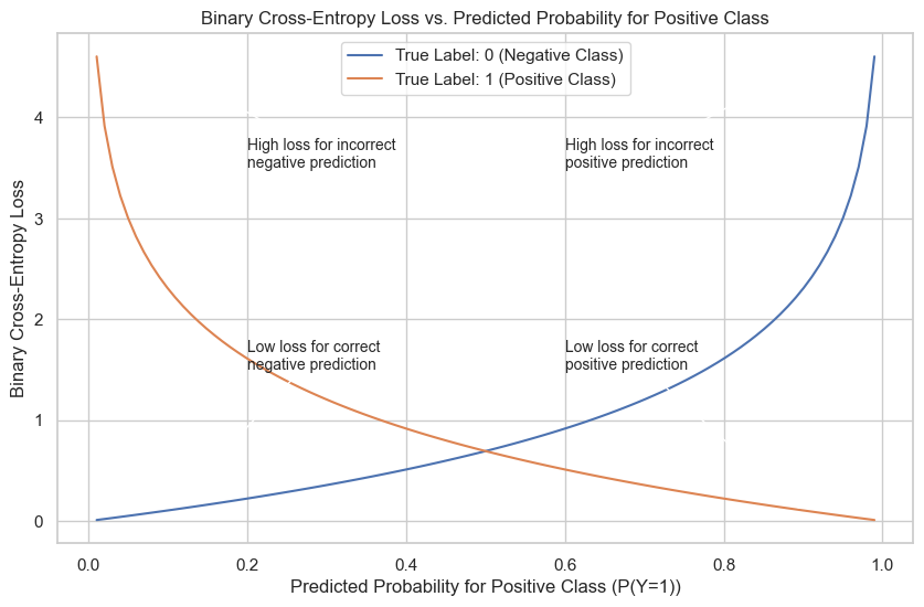
Categorical Cross-Entropy Plot Explanation
Implementing Categorical Cross-Entropy
Use the tf.keras.losses.CategoricalCrossentropy class to work with CCE in Keras. The function takes multiple parameters, including:
from_logits: A boolean value specifying whether to interpret y_pred as logits or probabilities.
label_smoothing: A float value in [0, 1] for label smoothing.
reduction: The type of tf.keras.losses.Reduction to apply to the loss.
Examples of Implementing CCE
To implement Categorical Cross-Entropy in Keras, you can either use the compile() API or as a standalone function.
Using the compile() API:
model.compile(optimizer=’sgd’, loss=tf.keras.losses.CategoricalCrossentropy())
As a standalone function:
y_true = [[0, 1, 0], [0, 0, 1]]
y_pred = [[0.05, 0.95, 0], [0.1, 0.8, 0.1]]
cce = tf.keras.losses.CategoricalCrossentropy()
cce(y_true, y_pred).numpy()
The Poison Loss
Poisson loss is a loss function often used in count-based regression problems. It computes the difference between the true count values and the predicted count values, making it suitable for tasks where the target variable represents the number of events occurring in a fixed interval of time or space.
Implementing Poisson Loss
To work with Poisson loss in Keras, use the tf.keras.losses.Poisson class. This function accepts the following parameters:
reduction: The type of tf.keras.losses.Reduction to apply to the loss. The default value is AUTO.
name: An optional name for the instance. Defaults to ‘poisson’.
Examples of Implementing Poisson Loss
You can implement Poisson loss in Keras using the compile() API or as a standalone function.
Using the compile() API:
model.compile(optimizer='sgd', loss=tf.keras.losses.Poisson())As a standalone function:
y_true = [[0., 1.], [0., 0.]]
y_pred = [[1., 1.], [0., 0.]]
# Using 'auto'/'sum_over_batch_size' reduction type.
p = tf.keras.losses.Poisson()
p(y_true, y_pred).numpy()

# Calling with 'sample_weight'.
p(y_true, y_pred, sample_weight=[0.8, 0.2]).numpy()

# Using 'sum' reduction type.
p = tf.keras.losses.Poisson(
reduction=tf.keras.losses.Reduction.SUM)
p(y_true, y_pred).numpy()
In the examples above, the Poisson loss is computed using different reduction types, demonstrating how you can customize the behavior of the loss function to suit your specific needs.
Kullback-Leibler Divergence Loss
Kullback-Leibler Divergence is a measure of how one probability distribution differs from a second, reference probability distribution. It is commonly used in machine learning to measure the difference between two probability distributions, typically in tasks such as unsupervised learning, anomaly detection, and information theory.
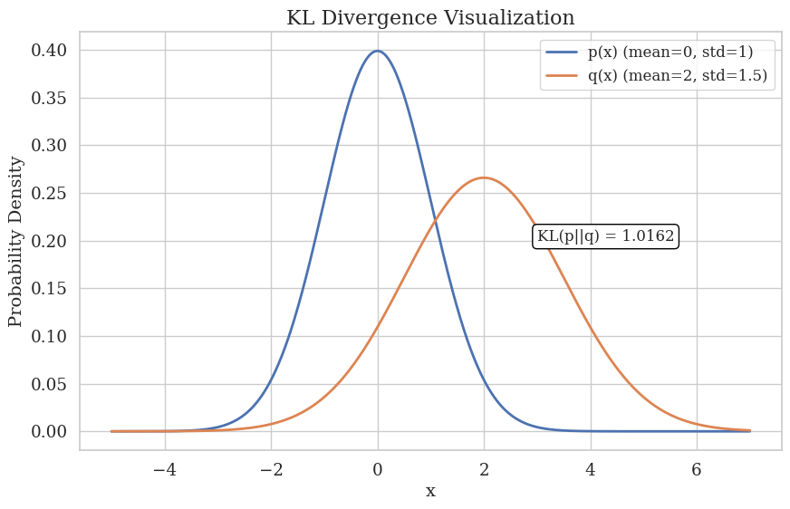
This visual representation demonstrates Kullback-Leibler (KL) divergence
Implementing Kullback-Leibler Divergence Loss
Use the tf.keras.losses.KLDivergence class to work with KL Divergence Loss in Keras. The function takes multiple parameters, including:
reduction: The type of tf.keras.losses.Reduction to apply to the loss.
name: The name for the operation (default is ‘kl_divergence’).
Examples of Implementing Kullback-Leibler Divergence Loss
To implement KL Divergence Loss in Keras, you can either use the compile() API or as a standalone function.
Using the compile() API:
model.compile(optimizer='sgd', loss=tf.keras.losses.KLDivergence())As a standalone function:
y_true = [[0, 1], [0, 0]]
y_pred = [[0.6, 0.4], [0.4, 0.6]]
kl = tf.keras.losses.KLDivergence()
kl(y_true, y_pred).numpy()
Mean Absolute Error
Mean Absolute Error (MAE) is a loss function that computes the mean of the absolute difference between labels (y_true) and predictions (y_pred). It is used for regression tasks, as it measures the average magnitude of errors between predicted and actual values, regardless of their direction. MAE is less sensitive to outliers compared to Mean Squared Error (MSE) and is a common metric for evaluating the performance of regression models.
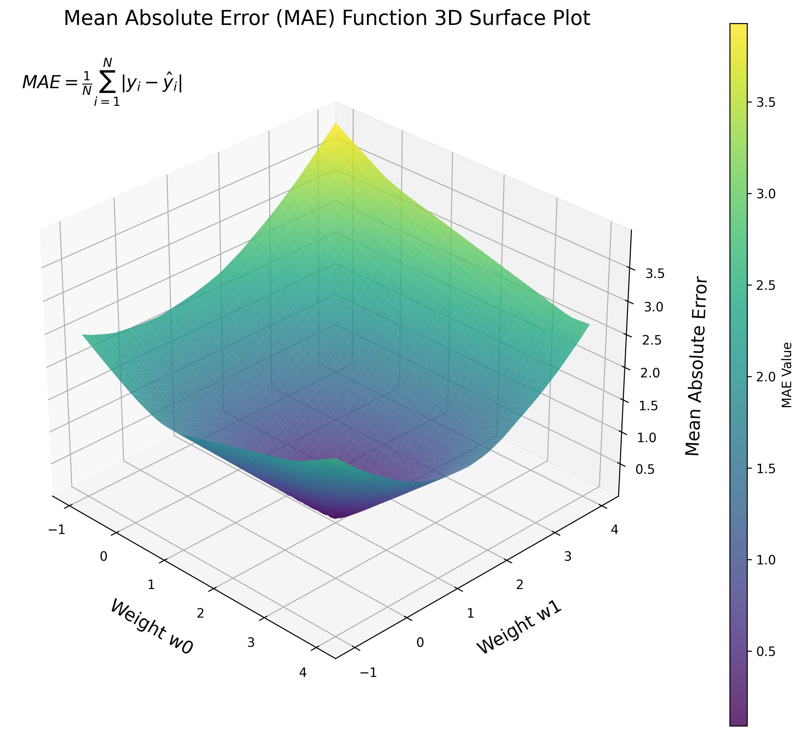
Implementing Mean Absolute Error
Use the tf.keras.losses.MeanAbsoluteError class to work with Mean Absolute Error in Keras. The function takes multiple parameters, including:
reduction: The type of tf.keras.losses.Reduction to apply to the loss.
name: The name for the operation (default is ‘mean_absolute_error’).
Examples of Implementing Mean Absolute Error
To implement Mean Absolute Error in Keras, you can either use the compile() API or as a standalone function.
Using the compile() API:
model.compile(optimizer='sgd', loss=tf.keras.losses.MeanAbsoluteError())As a standalone function:
y_true = [[0., 1.], [0., 0.]]
y_pred = [[1., 1.], [1., 0.]]
mae = tf.keras.losses.MeanAbsoluteError()
mae(y_true, y_pred).numpy()
Cosine Similarity Loss
Cosine Similarity is a measure of similarity between two non-zero vectors of an inner product space, which is widely used in information retrieval and natural language processing. It measures the cosine of the angle between two vectors, resulting in a value between -1 and 1. A value of -1 indicates a high degree of similarity, 1 indicates a high degree of dissimilarity, and 0 indicates orthogonality.
Implementing Cosine Similarity
Use the tf.keras.losses.CosineSimilarity class to work with Cosine Similarity in Keras. The function takes multiple parameters, including:
axis: The axis along which the cosine similarity is computed (default is -1).
reduction: The type of tf.keras.losses.Reduction to apply to the loss.
name: The name for the operation (default is ‘cosine_similarity’).
Examples of Implementing Cosine Similarity
To implement Cosine Similarity in Keras, you can either use the compile() API or as a standalone function.
Using the compile() API:
model.compile(optimizer='sgd', loss=tf.keras.losses.CosineSimilarity(axis=1))As a standalone function:
y_true = [[0., 1.], [1., 1.]]

y_pred = [[1., 0.], [1., 1.]]

cosine_loss = tf.keras.losses.CosineSimilarity(axis=1)

cosine_loss(y_true, y_pred).NumPy()
LogCosh Loss
Log-Cosh Loss is a loss function that computes the logarithm of the hyperbolic cosine of the prediction error (y_pred – y_true). It is used as a smooth approximation to the Mean Absolute Error (MAE), which makes it less sensitive to outliers in the data. This makes it suitable for use in regression tasks where there may be outliers or noisy data.
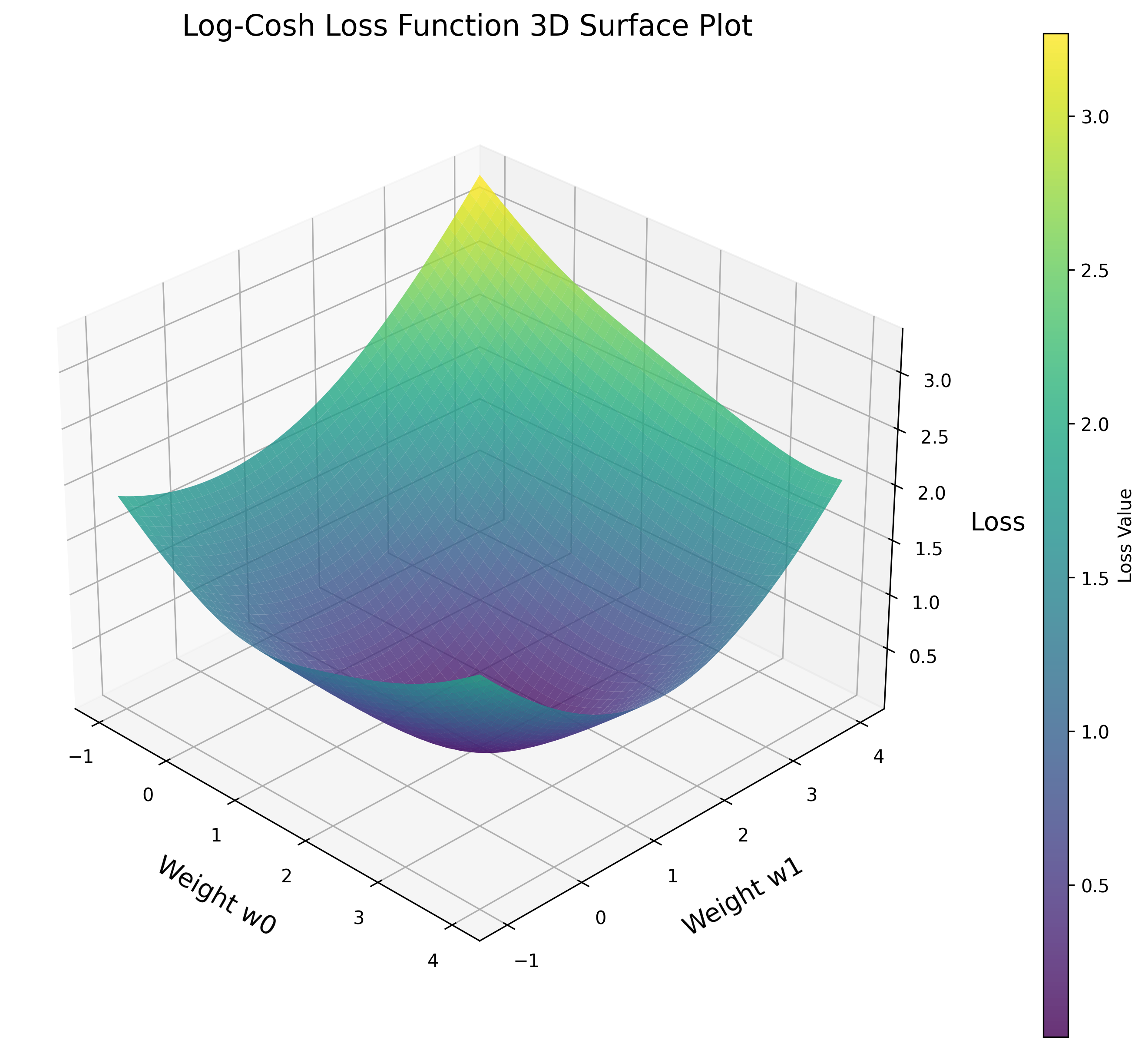

Implementing Log-Cosh Loss
Use the tf.keras.losses.LogCosh class to work with Log-Cosh Loss in Keras. The function takes multiple parameters, including:
reduction: The type of tf.keras.losses.Reduction to apply to the loss.
name: The name for the operation (default is ‘log_cosh’).
Examples of Implementing Log-Cosh Loss
To implement Log-Cosh Loss in Keras, you can either use the compile() API or as a standalone function.
Using the compile() API:
model.compile(optimizer='sgd', loss=tf.keras.losses.LogCosh())As a standalone function:
y_true = [[0., 1.], [0., 0.]]
y_pred = [[1., 1.], [0., 0.]]
l = tf.keras.losses.LogCosh()
l(y_true, y_pred).numpy()
Huber loss
Huber Loss is a loss function commonly used in regression problems that are less sensitive to outliers compared to Mean Squared Error (MSE). The Huber Loss function is quadratic for small errors and linear for large errors, making it more robust to outliers. This function has a parameter delta, which determines the point at which the loss function transitions from quadratic to linear. Huber Loss is widely used in robust regression and reinforcement learning.
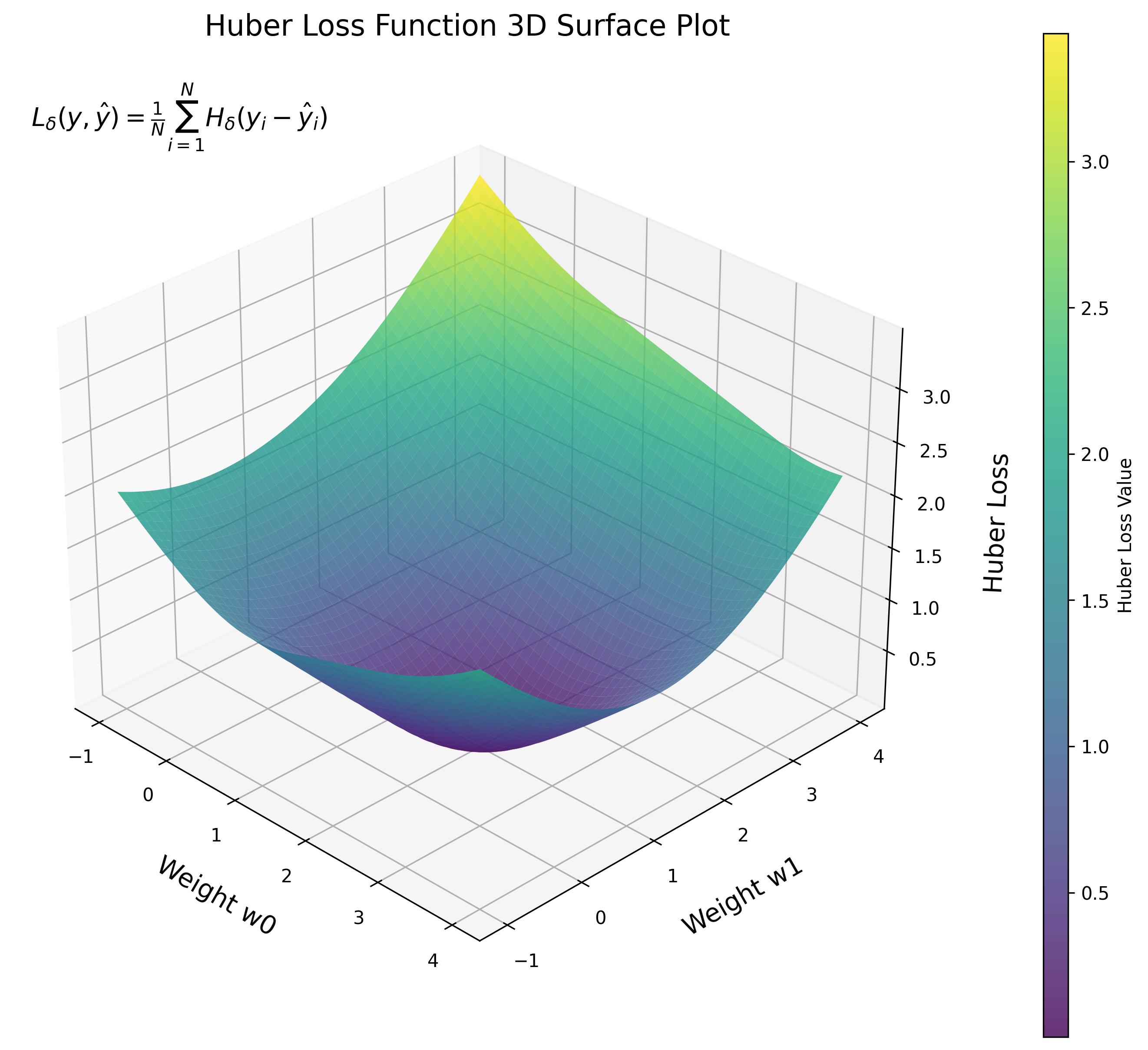
Implementing Huber Loss
Use the tf.keras.losses.Huber class to work with Huber Loss in Keras. The function takes multiple parameters, including:
Delta: A float representing the point where the Huber loss function transitions from quadratic to linear.
Reduction: The type of tf.keras.losses.Reduction to apply to the loss.
Name: The name for the operation (default is ‘huber_loss’).
Examples of Implementing Huber Loss
To implement Huber Loss in Keras, you can either use the compile() API or as a standalone function.
Using the compile() API:
model.compile(optimizer='sgd', loss=tf.keras.losses.Huber())As a standalone function:
y_true = [[0, 1], [0, 0]]

y_pred = [[0.6, 0.4], [0.4, 0.6]]

h = tf.keras.losses.Huber()

h(y_true, y_pred).numpy()
Learning Embeddings
Embeddings are a powerful technique used in machine learning to represent categorical variables as continuous vectors. They allow models to capture and learn relationships between categorical variables in a more expressive and meaningful manner. Keras provides a simple way to create and work with embeddings through the Embedding layer.
Here’s an example of how to use the Keras Embedding layer:
from tensorflow.keras.layers import Embedding

embedding_layer = Embedding(input_dim=1000, output_dim=64, input_length=10)
In this example, the input_dim parameter represents the number of unique categories in the input data (1000 in this case), output_dim is the size of the embedding vector (64), and input_length is the length of the input sequence (10).
Now that we’ve discussed embeddings, let’s dive into some loss functions that are suitable for learning embeddings. These loss functions can be particularly useful when working with complex data, such as images, text, or graphs.
Triplet Loss
Triplet loss is a popular loss function used to learn embeddings in tasks like face recognition, where the goal is to minimize the distance between an anchor and a positive example while maximizing the distance between the anchor and a negative example. The idea is to learn a function that can discriminate between positive and negative pairs effectively.
Here’s a simple example of how to implement triplet loss in Keras:
import tensorflow as tf

def triplet_loss(y_true, y_pred, alpha=0.2):
    anchor, positive, negative = tf.split(y_pred, num_or_size_splits=3, axis=1)

    positive_distance = tf.reduce_sum(tf.square(anchor - positive), axis=1)
    negative_distance = tf.reduce_sum(tf.square(anchor - negative), axis=1)

    loss = tf.maximum(positive_distance - negative_distance + alpha, 0.0)
    return tf.reduce_mean(loss)

model.compile(optimizer='adam', loss=triplet_loss)
In this example, the triplet_loss function takes the predicted embeddings for anchor, positive, and negative examples and computes the distances between them. The alpha parameter represents a margin that encourages the model to create a separation between positive and negative pairs.
Quadruplet loss is an extension of triplet loss and is similar to implementing triplet loss. It considers four embeddings: anchor, positive, negative, and another negative example from a different class than the anchor. The idea is to learn a function that can discriminate between positive and negative pairs more effectively by considering additional information.
Creating custom loss functions in Keras
In certain situations, the built-in loss functions provided by Keras may not be suitable for your specific problem. In such cases, you can create a custom loss function tailored to your needs. In this section, we will demonstrate how to create a custom loss function with a unique example that is both informative and applicable to real-world scenarios.
Example: Custom Loss Function for Balancing Precision and Recall
Suppose you are working on a binary classification problem where both false positives and false negatives carry significant costs. In this case, you might want to balance precision (the ability to correctly identify positive cases) and recall (the ability to identify all the actual positive cases) in your model.
To achieve this, you can create a custom F-beta loss function. The F-beta score is a metric that combines precision and recall using a parameter beta, which allows you to assign different weights to precision and recall. A higher beta value prioritizes recall, whereas a lower beta value emphasizes precision.
Here’s how you can define the custom F-beta loss function:
import keras.backend as K

def custom_fbeta_loss(y_true, y_pred, beta=1):
    # Calculate true positives, false positives, and false negatives
    true_positives = K.sum(y_true * y_pred)
    false_positives = K.sum((1 - y_true) * y_pred)
    false_negatives = K.sum(y_true * (1 - y_pred))

    # Calculate precision and recall
    precision = true_positives / (true_positives + false_positives + K.epsilon())
    recall = true_positives / (true_positives + false_negatives + K.epsilon())

    # Calculate the F-beta score and return its negative value as a loss
    fbeta_score = (1 + beta**2) * (precision * recall) / ((beta**2 * precision) + recall + K.epsilon())
    return 1 - fbeta_score
In this example, the parameter beta can be adjusted based on the specific requirements of your problem. The default value of beta is 1, which leads to the F1 score, a commonly used metric that balances precision and recall.
Once you have defined the custom loss function, you can use it in your model by passing it to the compile() method:
model.compile(loss=lambda y_true, y_pred: custom_fbeta_loss(y_true, y_pred, beta=1),
optimizer='adam')
In this unique example, we have demonstrated how to create a custom loss function that balances precision and recall for binary classification problems. By following these guidelines and adapting the example above, you can create custom loss functions that cater to the specific needs of your machine learning projects, providing both detailed and accurate content.
The add_loss() API
Handling Non-Standard Losses and Metrics with add_loss() Function in Keras
In most cases, losses and metrics can be computed using the true and predicted values (y_true and y_pred). However, there are situations where you might require a different approach. In this section, we’ll explore how to handle non-standard losses and metrics using Keras add_loss() function.
Consider a scenario where we want to add a custom layer to our model that penalizes the activation of a specific layer based on the L1 norm of its weights. This can help in encouraging sparse representations in our model.
Creating the L1 Penalty Layer
To create a custom layer with L1 penalty on weights, we will implement the following class:
import tensorflow as tf
from tensorflow.keras import layers

class L1PenaltyLayer(layers.Layer):
    def __init__(self, factor, **kwargs):
        super(L1PenaltyLayer, self).__init__(**kwargs)
        self.factor = factor

def call(self, inputs):
    l1_penalty = self.factor * tf.reduce_sum(tf.abs(inputs))
    self.add_loss(l1_penalty)
    return inputs
This custom layer calculates the L1 penalty on its input and adds the penalty as a loss using self.add_loss().
With the L1 penalty layer, the model will now encourage sparse representations in the first dense layer while training. The overall loss displayed during training will include both the sparse categorical cross-entropy loss and the L1 penalty loss.
Conclusion
In wrapping up, choosing the right loss function is essential to the success of your deep learning models. We’ve discussed various Keras loss functions, including Binary Cross Entropy, Poisson Loss, Kullback-Leibler Divergence Loss, and many others, along with practical examples to help you with their implementation.
Remember, the key is to grasp the differences between these loss functions and match them to your specific use cases. By doing so, you can make well-informed decisions and boost your model’s performance.
References
Lin, Tsung-Yi, et al. “Focal Loss for Dense Object Detection.” 2017 IEEE International Conference on Computer Vision (ICCV), IEEE, 2017, http://dx.doi.org/10.1109/iccv.2017.324. Accessed 15 May 2023.
“Scatter Plot with Quadratic Polynomial Regression Curve.” Plotly, https://chart-studio.plotly.com/~aayushmittalaayush/14/#/. Accessed 15 May 2023.
Team, Keras. Keras Documentation: Losses. https://keras.io/api/losses/. Accessed 15 May 2023.
Zhao, Xiaonan, et al. “A Weakly Supervised Adaptive Triplet Loss for Deep Metric Learning.” 2019 IEEE/CVF International Conference on Computer Vision Workshop (ICCVW), IEEE, 2019, http://dx.doi.org/10.1109/iccvw.2019.00393. Accessed 15 May 2023.


