Boost inference performance for Mixtral and Llama 2 models with new Amazon SageMaker containers

In January 2024, Amazon SageMaker launched a new version (0.26.0) of Large Model Inference (LMI) Deep Learning Containers (DLCs). This version offers support for new models (including Mixture of Experts), performance and usability improvements across inference backends, as well as new generation details for increased control and prediction explainability (such as reason for generation completion and token level log probabilities).

LMI DLCs offer a low-code interface that simplifies using state-of-the-art inference optimization techniques and hardware. LMI allows you to apply tensor parallelism; the latest efficient attention, batching, quantization, and memory management techniques; token streaming; and much more, by just requiring the model ID and optional model parameters. With LMI DLCs on SageMaker, you can accelerate time-to-value for your generative artificial intelligence (AI) applications, offload infrastructure-related heavy lifting, and optimize large language models (LLMs) for the hardware of your choice to achieve best-in-class price-performance.

In this post, we explore the latest features introduced in this release, examine performance benchmarks, and provide a detailed guide on deploying new LLMs with LMI DLCs at high performance.

New features with LMI DLCs

In this section, we discuss new features across LMI backends, and drill down on some others that are backend-specific. LMI currently supports the following backends:

• LMI-Distributed Library – This is the AWS framework to run inference with LLMs, inspired from OSS, to achieve the best possible latency and accuracy on the result
• LMI vLLM – This is the AWS backend implementation of the memory-efficient vLLM inference library
• LMI TensorRT-LLM toolkit – This is the AWS backend implementation of NVIDIA TensorRT-LLM, which creates GPU-specific engines to optimize performance on different GPUs
• LMI DeepSpeed – This is the AWS adaptation of DeepSpeed, which adds true continuous batching, SmoothQuant quantization, and the ability to dynamically adjust memory during inference
• LMI NeuronX – You can use this for deployment on AWS Inferentia2 and AWS Trainium-based instances, featuring true continuous batching and speedups, based on the AWS Neuron SDK

The following table sumarizes the newly added features, both common and backend-specific.

New models supported

New popular models are supported across backends, such as Mistral-7B (all backends), the MoE-based Mixtral (all backends except Transformers-NeuronX), and Llama2-70B (Transformers-NeuronX).

Context window extension techniques

Rotary Positional Embedding (RoPE)-based context scaling is now available on the LMI-Dist, vLLM, and TensorRT-LLM backends. RoPE scaling enables the extension of a model’s sequence length during inference to virtually any size, without the need for fine-tuning.

The following are two important considerations when using RoPE:

• Model perplexity – As the sequence length increases, so can the model’s perplexity. This effect can be partially offset by conducting minimal fine-tuning on input sequences larger than those used in the original training. For an in-depth understanding of how RoPE affects model quality, refer to Extending the RoPE.
• Inference performance – Longer sequence lengths will consume higher accelerator’s high bandwidth memory (HBM). This increased memory usage can adversely affect the number of concurrent requests your accelerator can handle.

Added generation details

You can now get two fine-grained details about generation results:

• finish_reason – This gives the reason for generation completion, which can be reaching the maximum generation length, generating an end-of-sentence (EOS) token, or generating a user-defined stop token. It is returned with the last streamed sequence chunk.
• log_probs – This returns the log probability assigned by the model for each token in the streamed sequence chunk. You can use these as a rough estimate of model confidence by computing the joint probability of a sequence as the sum of the log_probs of the individual tokens, which can be useful for scoring and ranking model outputs. Be mindful that LLM token probabilities are generally overconfident without calibration.

You can enable the generation results output by adding details=True in your input payload to LMI, leaving all other parameters unchanged:

payload = {“inputs”:“your prompt”,
“parameters”:{max_new_tokens”:256,...,“details”:True}
}

Consolidated configuration parameters

Finally, LMI configuration parameters have also been consolidated. For more information about all common and backend-specific deployment configuration parameters, see Large Model Inference Configurations.

LMI-Distributed backend

At AWS re:Invent 2023, LMI-Dist added new, optimized collective operations to speed up communication between GPUs, resulting in lower latency and higher throughput for models that are too big for a single GPU. These collectives are available exclusively for SageMaker, for p4d instances.

Whereas the previous iteration only supported sharding across all 8 GPUs, LMI 0.26.0 introduces support for a tensor parallel degree of 4, in a partial all-to-all pattern. This can be combined with SageMaker inference components, with which you can granularly configure how many accelerators should be allocated to each model deployed behind an endpoint. Together, these features provide better control over the resource utilization of the underlying instance, enabling you to increase model multi-tenancy by hosting different models behind one endpoint, or fine-tune the aggregate throughput of your deployment to match your model and traffic characteristics.

The following figure compares direct all-to-all with partial all-to-all.

TensorRT-LLM backend

NVIDIA’s TensorRT-LLM was introduced as part of the previous LMI DLC release (0.25.0), enabling state-of-the-art GPU performance and optimizations like SmoothQuant, FP8, and continuous batching for LLMs when using NVIDIA GPUs.

TensorRT-LLM requires models to be compiled into efficient engines before deployment. The LMI TensorRT-LLM DLC can automatically handle compiling a list of supported models just-in-time (JIT), before starting the server and loading the model for real-time inference. Version 0.26.0 of the DLC grows the list of supported models for JIT compilation, introducing Baichuan, ChatGLM , GPT2, GPT-J, InternLM, Mistral, Mixtral, Qwen, SantaCoder and StarCoder models.

JIT compilation adds several minutes of overhead to endpoint provisioning and scaling time, so it is always recommended to compile your model ahead-of-time. For a guide on how to do this and a list of supported models, see TensorRT-LLM ahead-of-time compilation of models tutorial. If your selected model isn’t supported yet, refer to TensorRT-LLM manual compilation of models tutorial to compile any other model that is supported by TensorRT-LLM.

Additionally, LMI now exposes native TensorRT-LLM SmootQuant quantization, with parameters to control alpha and scaling factor by token or channel. For more information about the related configurations, refer to TensorRT-LLM.

vLLM backend

The updated release of vLLM included in LMI DLC features performance improvements of up to 50% fueled by CUDA graph mode instead of eager mode. CUDA graphs accelerate GPU workloads by launching several GPU operations in one go instead of launching them individually, which reduces overheads. This is particularly effective for small models when using tensor parallelism.

The added performance comes at a trade-off of added GPU memory consumption. CUDA graph mode is now default for the vLLM backend, so if you are constrained on the amount of GPU memory available, you can set option.enforce_eager=True to force PyTorch eager mode.

Transformers-NeuronX backend

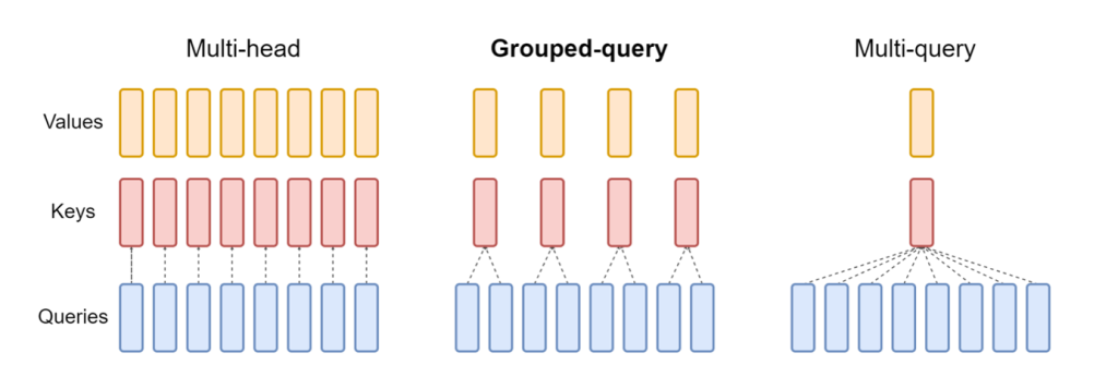
The updated release of NeuronX included in the LMI NeuronX DLC now supports models that feature the grouped-query attention mechanism, such as Mistral-7B and LLama2-70B. Grouped-query attention is an important optimization of the default transformer attention mechanism, where the model is trained with fewer key and value heads than query heads. This reduces the size of the KV cache on GPU memory, allowing for greater concurrency, and improving price-performance.

The following figure illustrates multi-head, grouped-query, and multi-query attention methods (source).

Different KV cache sharding strategies are available to suit different types of workloads. For more information on sharding strategies, see Grouped-query attention (GQA) support. You can enable your desired strategy (shard-over-heads, for example) with the following code:

option.group_query_attention=shard-over-heads

Additionally, the new implementation of NeuronX DLC introduces a cache API for TransformerNeuronX that enables access to the KV cache. It allows you to insert and remove KV cache rows from new requests while you’re handing batched inference. Before introducing this API, the KV cache was recomputed for any newly added requests. Compared to LMI V7 (0.25.0), we have improved latency by more than 33% with concurrent requests, and support much higher throughput.

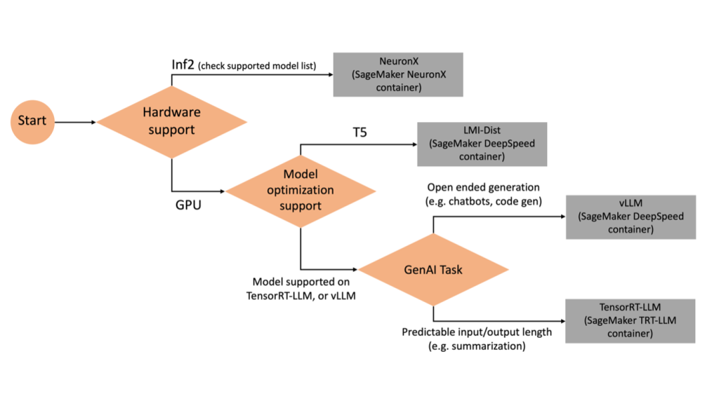
Selecting the right backend

To decide what backend to use based on the selected model and task, use the following flow chart. For individual backend user guides along with supported models, see LMI Backend User Guides.

Deploy Mixtral with LMI DLC with additional attributes

Let’s walk through how you can deploy the Mixtral-8x7B model with LMI 0.26.0 container and generate additional details like log_prob and finish_reason as part of the output. We also discuss how you can benefit from these additional attributes through a content generation use case.

The complete notebook with detailed instructions is available in the GitHub repo.

We start by importing the libraries and configuring the session environment:

import boto3
import sagemaker 
import json 
import io 
import numpy as np 
from sagemaker import Model, image_uris, serializers, deserializers 

role = sagemaker.get_execution_role() # execution role for the endpoint 
session = sagemaker.session.Session() # sagemaker session for interacting with different AWS APIs 
region = session._region_name # region name of the current SageMaker Studio environment

You can use SageMaker LMI containers to host models without any additional inference code. You can configure the model server either through the environment variables or a serving.properties file. Optionally, you could have a model.py file for any preprocessing or postprocessing and a requirements.txt file for any additional packages that are required to be installed.

In this case, we use the serving.properties file to configure the parameters and customize the LMI container behavior. For more details, refer to the GitHub repo. The repo explains details of the various configuration parameters that you can set. We need the following key parameters:

• engine – Specifies the runtime engine for DJL to use. This drives the sharding and the model loading strategy in the accelerators for the model.
• option.model_id – Specifies the Amazon Simple Storage Service (Amazon S3) URI of the pre-trained model or the model ID of a pretrained model hosted inside a model repository on Hugging Face. In this case, we provide the model ID for the Mixtral-8x7B model.
• option.tensor_parallel_degree – Sets the number of GPU devices over which Accelerate needs to partition the model. This parameter also controls the number of workers per model that will be started up when DJL serving runs. We set this value to max (maximum GPU on the current machine).
• option.rolling_batch – Enables continuous batching to optimize accelerator utilization and overall throughput. For the TensorRT-LLM container, we use auto.
• option.model_loading_timeout – Sets the timeout value for downloading and loading the model to serve inference.
• option.max_rolling_batch – Sets the maximum size of the continuous batch, defining how many sequences can be processed in parallel at any given time.

%%writefile serving.properties 
engine=MPI 
option.model_id=mistralai/Mixtral-8x7B-v0.1 
option.tensor_parallel_degree=max 
option.max_rolling_batch_size=32 
option.rolling_batch=auto 
option.model_loading_timeout = 7200

We package the serving.properties configuration file in the tar.gz format, so that it meets SageMaker hosting requirements. We configure the DJL LMI container with tensorrtllm as the backend engine. Additionally, we specify the latest version of the container (0.26.0).

image_uri = image_uris.retrieve(
   framework="djl-tensorrtllm",
   region=sess.boto_session.region_name,
   version="0.26.0"
)

Next, we upload the local tarball (containing the serving.properties configuration file) to an S3 prefix. We use the image URI for the DJL container and the Amazon S3 location to which the model serving artifacts tarball was uploaded, to create the SageMaker model object.

model = Model(image_uri=image_uri, model_data=code_artifact, role=role) 

instance_type = "ml.p4d.24xlarge" 
endpoint_name = sagemaker.utils.name_from_base("mixtral-lmi-model") 

model.deploy(
   initial_instance_count=1,
   instance_type=instance_type,
   endpoint_name=endpoint_name,
   container_startup_health_check_timeout=1800
)

As part of LMI 0.26.0, you can now use two additional fine-grained details about the generated output:

• log_probs – This is the log probability assigned by the model for each token in the streamed sequence chunk. You can use these as a rough estimate of model confidence by computing the joint probability of a sequence as the sum of the log probabilities of the individual tokens, which can be useful for scoring and ranking model outputs. Be mindful that LLM token probabilities are generally overconfident without calibration.
• finish_reason – This is the reason for generation completion, which can be reaching the maximum generation length, generating an EOS token, or generating a user-defined stop token. This is returned with the last streamed sequence chunk.

You can enable these by passing "details"=True as part of your input to the model.

Let’s see how you can generate these details. We use a content generation example to understand their application.

We define a LineIterator helper class, which has functions to lazily fetch bytes from a response stream, buffer them, and break down the buffer into lines. The idea is to serve bytes from the buffer while fetching more bytes from the stream asynchronously.

class LineIterator:
    def __init__(self, stream):
        # Iterator to get bytes from stream 
        self.byte_iterator = iter(stream)  
        # Buffer stream bytes until we get a full line
        self.buffer = io.BytesIO()  
        # Track current reading position within buffer
        self.read_pos = 0

   def __iter__(self):
        # Make class iterable 
        return self

    def __next__(self):
        while True:
           # Seek read position within buffer
           self.buffer.seek(self.read_pos)  
           # Try reading a line from current position
           line = self.buffer.readline()
           # If we have a full line
           if line and line[-1] == ord('n'):
               # Increment reading position past this line
               self.read_pos += len(line)  
               # Return the line read without newline char
               return line[:-1] 
           # Fetch next chunk from stream  
           try:
               chunk = next(self.byte_iterator)
           # Handle end of stream 
           except StopIteration:
               # Check if we have any bytes still unread
               if self.read_pos < self.buffer.getbuffer().nbytes:
                   continue
               # If not, raise StopIteration
               raise
           # Add fetched bytes to end of buffer
           self.buffer.seek(0, io.SEEK_END)  
           self.buffer.write(chunk['PayloadPart']['Bytes'])

Generate and use token probability as an additional detail

Consider a use case where we are generating content. Specifically, we’re tasked with writing a brief paragraph about the benefits of exercising regularly for a lifestyle-focused website. We want to generate content and output some indicative score of the confidence that the model has in the generated content.

We invoke the model endpoint with our prompt and capture the generated response. We set "details": True as a runtime parameter within the input to the model. Because the log probability is generated for each output token, we append the individual log probabilities to a list. We also capture the complete generated text from the response.

sm_client = boto3.client("sagemaker-runtime")

# Set details: True as a runtime parameter within the input.
body = {"inputs": prompt, "parameters": {"max_new_tokens":512, "details": True}}
resp = sm_client.invoke_endpoint_with_response_stream(EndpointName=endpoint_name, Body=json.dumps(body), ContentType="application/json")
event_stream = resp['Body']

overall_log_prob = []

for line in LineIterator(event_stream):
    resp = json.loads(line)
    if resp['token'].get('text') != None:
        token_log_prob = resp['token']['log_prob']
        overall_log_prob.append(token_log_prob)
    elif resp['generated_text'] != None:
        generated_text= resp['generated_text']

To calculate the overall confidence score, we calculate the mean of all the individual token probabilities and subsequently get the exponential value between 0 and 1. This is our inferred overall confidence score for the generated text, which in this case is a paragraph about the benefits of regular exercising.

print(generated_text) 
overall_score=np.exp(np.mean(overall_log_prob)) 
print(f"nnOverall confidence score in the generated text: {overall_score}")

This was one example of how you can generate and use log_prob, in the context of a content generation use case. Similarly, you can use log_prob as measure of confidence score for classification use cases.

Alternatively, you can use it for the overall output sequence or sentence-level scoring to evaluate the affect of parameters such as temperature on the generated output.

Generate and use finish reason as an additional detail

Let’s build on the same use case, but this time we’re tasked with writing a longer article. Additionally, we want to make sure that the output is not truncated due to generation length issues (max token length) or due to stop tokens being encountered.

To accomplish this, we use the finish_reason attribute generated in the output, monitor its value, and continue generating until the entire output is generated.

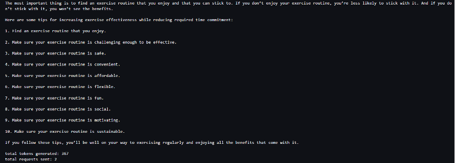
We define an inference function that takes a payload input and calls the SageMaker endpoint, streams back a response, and processes the response to extract generated text. The payload contains the prompt text as inputs and parameters like max tokens and details. The response is read in a stream and processed line by line to extract the generated text tokens into a list. We extract details like finish_reason. We call the inference function in a loop (chained requests) while adding more context each time, and track the number of tokens generated and number of requests sent until the model finishes.

def inference(payload):
    # Call SageMaker endpoint and get response stream
    resp = sm_client.invoke_endpoint_with_response_stream(EndpointName=endpoint_name, Body=json.dumps(payload), ContentType="application/json")
    event_stream = resp['Body']
    text_output = []
    for line in LineIterator(event_stream):
        resp = json.loads(line) 
        # Extract text tokens if present
        if resp['token'].get('text') != None:
            token = resp['token']['text']
            text_output.append(token)  
            print(token, end='')
        # Get finish reason if details present
        if resp.get('details') != None:
            finish_reason = resp['details']['finish_reason']
            # Return extracted output, finish reason and token length
            return payload['inputs'] + ''.join(text_output), finish_reason, len(text_output)

# set details: True as a runtime parameter within the input.
payload = {"inputs": prompt,  "parameters": {"max_new_tokens":256, "details": True}} 

finish_reason = "length"
# Print initial output 
print(f"Output: {payload['inputs']}", end='')  
total_tokens = 0
total_requests = 0
while finish_reason == 'length':
    # Call inference and get extracts
    output_text, finish_reason, out_token_len = inference(payload)
    # Update payload for next request
    payload['inputs'] = output_text 
    total_tokens += out_token_len
    total_requests += 1
# Print metrics
print(f"nntotal tokens generated: {total_tokens} ntotal requests sent: {total_requests}")

As we can see, even though the max_new_token parameter is set to 256, we use the finish_reason detail attribute as part of the output to chain multiple requests to the endpoint, until the entire output is generated.

Similarly, based on your use case, you can use stop_reason to detect insufficient output sequence length specified for a given task or unintended completion due to a human stop sequence.

Conclusion

In this post, we walked through the v0.26.0 release of the AWS LMI container. We highlighted key performance improvements, new model support, and new usability features. With these capabilities, you can better balance cost and performance characteristics while providing a better experience to your end-users.

To learn more about LMI DLC capabilities, refer to Model parallelism and large model inference. We’re excited to see how you use these new capabilities from SageMaker.

About the authors

João Moura is a Senior AI/ML Specialist Solutions Architect at AWS. João helps AWS customers – from small startups to large enterprises – train and deploy large models efficiently, and more broadly build ML platforms on AWS.

Rahul Sharma is a Senior Solutions Architect at AWS, helping AWS customers design and build AI/ML solutions. Prior to joining AWS, Rahul has spent several years in the finance and insurance sector, helping customers build data and analytical platforms.

Qing Lan is a Software Development Engineer in AWS. He has been working on several challenging products in Amazon, including high performance ML inference solutions and high performance logging system. Qing’s team successfully launched the first Billion-parameter model in Amazon Advertising with very low latency required. Qing has in-depth knowledge on the infrastructure optimization and Deep Learning acceleration.

Jian Sheng is a Software Development Engineer at Amazon Web Services who has worked on several key aspects of machine learning systems. He has been a key contributor to the SageMaker Neo service, focusing on deep learning compilation and framework runtime optimization. Recently, he has directed his efforts and contributed to optimizing the machine learning system for large model inference.

Tyler Osterberg is a Software Development Engineer at AWS. He specializes in crafting high-performance machine learning inference experiences within SageMaker. Recently, his focus has been on optimizing the performance of Inferentia Deep Learning Containers on the SageMaker platform. Tyler excels in implementing performant hosting solutions for large language models and enhancing user experiences using cutting-edge technology.

Rupinder Grewal is a Senior AI/ML Specialist Solutions Architect with AWS. He currently focuses on serving of models and MLOps on Amazon SageMaker. Prior to this role, he worked as a Machine Learning Engineer building and hosting models. Outside of work, he enjoys playing tennis and biking on mountain trails.

Dhawal Patel is a Principal Machine Learning Architect at AWS. He has worked with organizations ranging from large enterprises to mid-sized startups on problems related to distributed computing, and Artificial Intelligence. He focuses on Deep learning including NLP and Computer Vision domains. He helps customers achieve high performance model inference on SageMaker.

Raghu Ramesha is a Senior ML Solutions Architect with the Amazon SageMaker Service team. He focuses on helping customers build, deploy, and migrate ML production workloads to SageMaker at scale. He specializes in machine learning, AI, and computer vision domains, and holds a master’s degree in Computer Science from UT Dallas. In his free time, he enjoys traveling and photography.